5 minutes
Logistic Regression from scratch
Fundamentals
Logistic Regression models, unlike Linear Regression, should help us predict the probability of a given outcome - e.g. if a payment is fraudulent or not. A Logistic Regression model, just like in Linear Regression can be represented as follows:
$$ \text{z} = \text{b} + w_1 x_1 + w_2 x_2 + \dots + w_n x_n $$- \(\text{z}\) is the output of the linear equation, also called the log odds.
- \(\text{b}\) is the bias.
- The \(w_i\) values are the model’s learned weights.
- The \(x_i\) values are the feature values for a particular example.
However we need to keep in mind that the output needs to be represented as a probability instead, i.e. a value between 0 and 1. This is where log-odds come in.
Let’s start by understanding what odds are.
Odds
The odds of an event are calculated as the probability of the event occurring divided by the probability of the event not occurring \((p / (1-p))\).
Odds are not probabilities, but the ratio of something happening vs the ratio of something not happening. Probabilities are the ratio of something happening to everything that could happen.
Example could be odds of a given team winning a game are 5:3, so 5/3 = 1.7. The probability of the team winning the same is 5/(5+3) = 5/8 = 0.625.
Log-odds
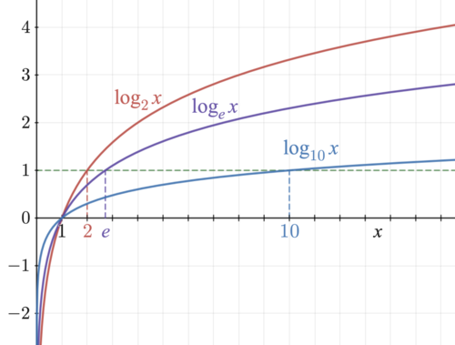
The odds of a team losing will always be a number from 0 to 1, e.g. 1/3 or 1/20 or 1/100. While the odds of a team winning will always be a number from 1 to \((+\infty\)) - this creates asymmetry. This is where log(odds) comes into play, as by doing the log of the odds everything becomes symmetrical instead!
Let’s consider two examples:
- ratio of 1 to 6: log(1/6) = log(0.17) = -1.79
- ratio of 6 to 1: log(6/1) = log(6) = 1.79
So if the logs are against, the log(odds) will be negative up to infinity, while if they are in favor we see the opposite. By using the log function we ensure that the distance from the origin (0) is the same for 1:6 and 6:1, which wouldn’t be possible otherwise.
The log-odds is the natural logarithm of the odds, expressed as:
$$ \text{logit}(p) = \log\left(\frac{p}{1 - p}\right) $$Sigmoid function
To go from log-odds back to probability, we can use the sigmoid function:
$$ \text{y'} = \frac{1}{1 + e^{-z}} $$Something worth keeping in mind is that the linear function from the logistic regression model becomes input to the sigmoid function, which turns it into a s-shape function. The log-odds are transformed from really large numbers of z into probabilities between 0 and 1, exclusive.
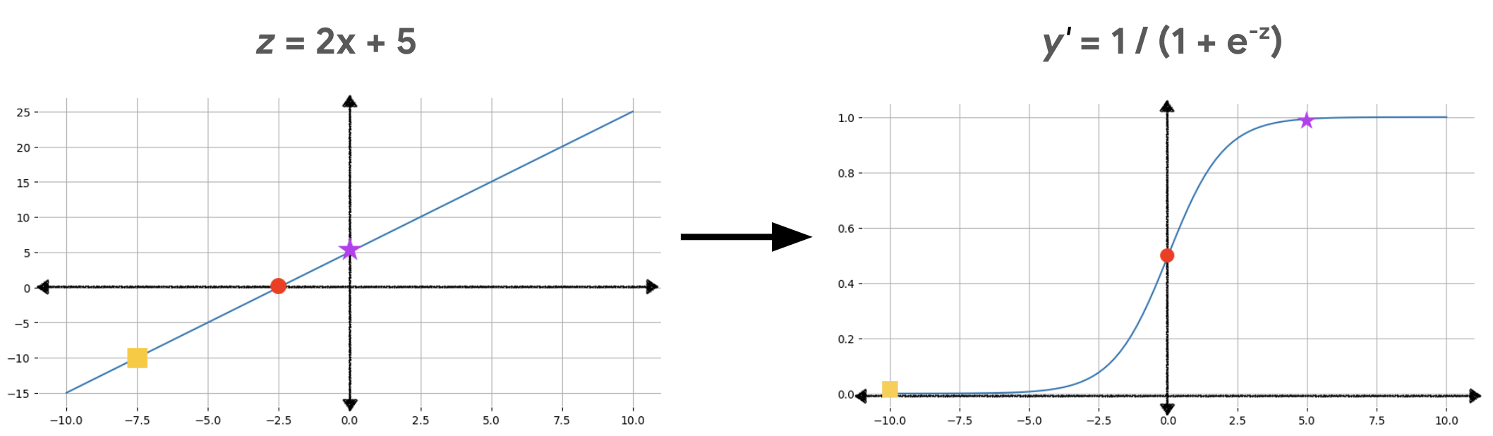
So essentially the output of a logistic regression model is a log-odds, which can easily be transformed into a probability through the sigmoid function.
Loss Functions: Log loss
The Log Loss equation returns the logarithm of the magnitude of the change, rather than just the distance from data to prediction.
$$ \text{LogLoss}(y, \hat{y}) = - \left( y \cdot \log(\hat{y}) + (1 - y) \cdot \log(1 - \hat{y}) \right) $$It’s worth understanding what would happen if we used the same loss function as a linear regression model, e.g. MSE. Let’s assume we have 3 models - A, B and C, predicting 0.9, 0.6 and 0.0001, respectively for a true label example.
Model A
$$ \text{MSE} = (0.9 - 1)^2 = 0.01 $$ $$ \text{LogLoss} = -\left(1 \cdot \log(0.9) + 0 \cdot \log(1 - 0.9)\right) = -\log(0.9) \approx 0.105 $$Model B
$$ \text{MSE} = (0.6 - 1)^2 = 0.16 $$ $$ \text{LogLoss} = -\log(0.6) \approx -0.22 $$Model C
$$ \text{MSE} = (0.0001 - 1)^2 \approx 0.99 $$ $$ \text{LogLoss} = -\log(0.0001) = -4 $$The difference in MSE for models A and B is just 0.15, which is incredibily small, even though model B is not doing a good job. MSE only sees “how close is the number to 1”, and 0.6 is numerically closer to 1 than, say, 0.2. It doesn’t understand that 0.6 means “not very confident”.
It’s also possible to see in model C what happens when the model is incredibily wrong, for the possible label (y=1) the log loss becomes:
$$ \text{LogLoss} = -\log(\hat{y}) $$So if the prediction is close to 0, the loss is going to be increasing towards \((+\infty\)). It’s always worth checking how the log function works, for values from 1 and 0 in the x axis, y decreases rapidily, which is exactly what we are seeing here (although the inverse since the loss function is \(-\log(\text{x})\)). On the other hand, if the prediction is close to 1, the loss is going get closer to 0, as \(~log(1) = 0\).
Similarly, when predicting the negative label, it becomes:
$$ \text{LogLoss} = -\log(1 - \hat{y}) $$So the log loss is essentially \(-\log(\hat{y})\) if y = 1 or \(-\log(1 - \hat{y})\) if y = 0, which makes it quite straightforward to understand.
Recap
| Concept | Equation | Meaning |
|---|---|---|
| Linear model | \( z = w \cdot x + b \) | Weighted sum of inputs |
| Log-odds | \( \log\left( \frac{p}{1 - p} \right) = z \) | The linear model predicts log-odds. The log-odds scale is unbounded (\(-\infty\) to \(+\infty\)) perfect for linear models |
| Probability (sigmoid) | \( p = \frac{1}{1 + e^{-z}} \) | Converts log-odds to probability. Probability scale is bounded (0 to 1) |
| Log loss | \( -y \log(\hat{p}) - (1 - y) \log(1 - \hat{p}) \) | Penalizes confident wrong predictions |