13 minutes
Brand Recommendations - TF-IDF
I started learning about Machine Learning with a couple online courses. The thing with these courses is that I got to learn a lot of cool stuff supported with step-by-step tutorials, but I never took some time to actually build something on my own, that tackles a real issue that I’m facing.
This is where things get interesting. One of the initiatives that I had at the company I was working back then was around brand recommendations. So I started wondering how hard could it be to build a simple machine learning model to provide brand recommendations.
This blog post will describe all the steps that were taken to build a baseline model that provides brand recommendations for the top brands available on well knwon e-commerce marketplace. Please note that the approach used here is not rocket science.
How does a recommendations system work?
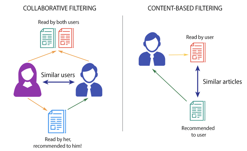
I will start by briefly explaining how the two most common types of recommendation systems work. Let’s consider the example of a platform like Medium that has to recommend articles to users. It can either recommend articles to users based on their content, or based on what similar users tend to read.
-
Collaborative Filtering: providing article recommendations based on what other similar users also read. Based on the interactions that users have with the same articles, the system provides article recommendations with more confidence
-
Content-Based Filtering: providing article recommendations based on the content of the article. If users usually read articles about machine learning, they will be more likely to read other articles that share the same topic
Even though I find the Collaborative Filtering type of systems a lot more interesting, they are generally more challenging. I decided to start with a Content-Based Recommendations System as the only data that it will need are descriptions from products available on the website. Later on, I will consider building a Hybrid Recommendations System where both Content-Based and Collaborative Filtering can be used simultaneously.
The goal will be to build a Content-Based Brand Recommendations System that provides the Top N brand recommendations for a particular brand.
Term Frequency - Inverse Document Frequency
TF-IDF stands for Term Frequency - Inverse Document Frequency and is used to measure how important a keyword (or multiple keywords) is to a document in a collection of documents (e.g. blog posts on this website). TF-IDF is the product of two different frequencies:
-
Term Frequency: measures how frequent a term is in a document. It will increase if the number of times a term appears also increases.
TF(t) = Number of times term t appears in a document / Total number of terms in the document -
Inverse Document Frequency: measures how important a term is. It will increase if the number of documents that contain the term decreases, i.e. if a term is rare. Meaning that common English words (e.g. the, or, a) should be quite irrelevant as they will be common on all the documents (as long as those documents are written in English). On the other hand, if we consider all the articles on my blog, words like brand, recommendations and machine-learning will be particularly relevant for the article you are reading.
IDF(t) = log(Total number of documents / Number of documents with term t in it)The logarithm is used to smooth the impact that higher values can have in the Inverse Document Frequency. Let’s remove the
logfor a moment and consider a corpus that consists of one million documents where only one of them contains the term machine-learning. In this scenario we would have 1.000.000/1, thus an Inverse Document Frequency of 1.000.000, which in turn would make the Term Frequency completely useless.
TF-IDF = TF x IDF
TF-IDF will give us the weight that each term has w.r.t. each particular document. We will consider each document to be a different brand. For each brand, we will build a brand description by merging some of their product descriptions. For the brand Adidas, we will bring together the descriptions of up to N products - stan smith, ultra boost, etc - and combine them into a brand description.
| Term A | Term B | Term C | |
|---|---|---|---|
| Brand A | |||
| Brand B |
The result will be a N_brands x N_terms matrix, where each row is a vector that represents a given brand - (weight_term_A, weight_term_B, weight_term_C). We won’t be able to find which brands are related by only looking at this matrix. Instead, we need to find a way to build a matrix that compares each brand to every other brand - N_brands x N_brands - and this is where Cosine Similarities come in handy.
| Brand A | Brand B | |
|---|---|---|
| Brand A | ||
| Brand B |
Cosine Similarity
Well, we already have a vector for each of the brands. It’s time to compare them to see which vectors are similar. Cosine Similarity is one of the most common strategies to compare how similar two vectors are. It is defined by the cosine of the angle between two vectors, and we will see later that it should be the same as the dot product of the two vectors when they are normalized, i.e. both have length 1.
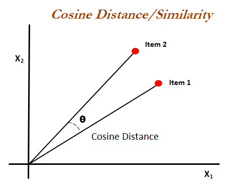
Even though the cosine values range from -1 to 1, we will never have negative values in our vectors. The range will always be from 0 to 1, where values near 1 will mean that the vectors are similar, i.e. the brands that those vectors correspond to are similar and can be recommended together.
The easiest way to see this in practice is to consider two vectors that denote the same brand, which is the same as saying two equal vectors. If they are the same, then the angle between the two is 0. The cosine of its angle cos(0) is 1. When building our N_brands x N_brands matrix, we will see that, for each brand, the most similar brand (where the cosine similarity is 1) is the brand itself.
| Brand A | Brand B | |
|---|---|---|
| Brand A | 1 | ? |
| Brand B | ? | 1 |
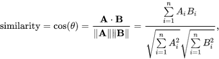
Let’s now look at the cosine similarity formula. If our vectors are normalized, every vector has length 1, meaning that we can remove the fraction’s denominator as it will also be 1. Without the denominator, the only thing left to calculate is the dot product of the vectors we want to compare.
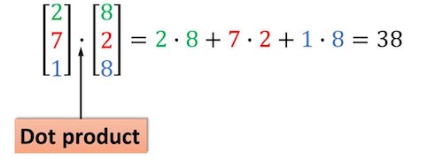
If you look closely, the dot product should be straightforward, as each Ai x Bi will be the multiplication of the weights of the term i for the brands A and B. The image below should help understanding how the dot product of two vectors works.
So, for each brand, we will calculate the dot product that the brand’s vector makes with every other brand’s vector, which will result in the N_brands x N_brands matrix that we were seeking. To provide the Top N recommendations for a given brand, we will have to search for the brands that resulted in a higher dot product for the brand we are testing.
Looking at the example below, we can see that we would be more likely to recommend brand C (0.8) than brand B (0.1) to users that also like or buy products from brand A.
| Brand A | Brand B | Brand C | |
|---|---|---|---|
| Brand A | 1 | 0.1 | 0.8 |
| Brand B | 0.1 | 1 | 0.3 |
| Brand C | 0.8 | 0.3 | 1 |
Step by step
Now that we have gone through the theory of how both TF-IDF and Cosine Similarities work, we can start describing step-by-step how to build the recommendations model. All the code described below is available in a Github repository.
Gather Data
The first step was to gather the data that the model will be trained with. For the sake of simplicity let’s assume that we had access to the data in a Neo4j instance. The data (brands, products and their descriptions) is available on the website and could be easily retrieved with a scrapper and then loaded into Neo4j.
The e-commerce website has thousands of brands available. It’s critical to filter a subset of brands that can be appropriate for the model. I have concluded that it would be worth filtering the brands with a significant number of products, e.g. at least 1000 products. Funny enough, the result is around 1000 brands as well.
from neo4j import GraphDatabase

db = GraphDatabase.driver("bolt://hostname:port", auth=(username, password))

MIN_PRODUCTS = 1000

statement = f"""
MATCH (brand:Brand)-[has_product:HAS_PRODUCT]->(product:Product)
WHERE count(has_product) > {MIN_PRODUCTS}
RETURN brand
"""

brands = db.session().run(statement)
filtered_brand_ids = [brand['brandId']) for brand in brands]

print(f"Total filtered brands: {len(filtered_brand_ids)}")
As soon as we have the brands that will be used by our model, it’s time to gather the descriptions from up to 20000 of their products. A CSV file is created with the brand identifiers (id and name) and their corresponding description - i.e. the result of merging the descriptions from their products.
Keep in mind that concatenating all the product descriptions into a single brand description is naïve. In the future, we could reconsider and replace it with a better strategy.
from collections import defaultdict

statement = """
MATCH (brand:Brand { brandId: $id })-[has_product:HAS_PRODUCT]->(product:Product)
WITH collect(product.description)[0..20000] as descriptions, brand
RETURN brand, descriptions
"""

# create a session to run all the neo4j queries
session = db.session()

brand_descriptions = defaultdict(list)

f = open('brand_descriptions.csv', 'w')

# csv file with: brand id, brand name, brand description
f.write("brand_id,brand_name,description\\n")

for brand_id in filtered_brand_ids:
    brand_descriptions_neo4j = session.run(statement, id=brand_id)

    for brand, descriptions in brand_descriptions_neo4j:
        brand_name = brand['name']
        brand_descriptions[brand_id] = descriptions

    # concat product descriptions to build the brand description
    concated_descriptions = ' '.join(brand_descriptions[brand_id])

    # pre-process descriptions
  	brand_description = pre_process(concated_descriptions)

    f.write(f"{brand_id},{brand_name},\\"{str(brand_description)}\\" \\n")
f.close()
Preparing the data
You might have noticed that each brand description is processed right before being written to the resulting CSV file.
There was nothing special when it comes to preparing the data. We are just replacing some special characters on the product descriptions to avoid having them on the final brand description, as they don’t add any value. When training the model, we will also make sure to remove the most common English words (e.g. a, or, the) since they don’t add any value either.
Finally, we convert all the text to lowercase since terms like Red, and red shouldn’t be any different.
import numpy as np

def pre_process(brand_description):
    # pontuaction
    symbols = "!\\"#$%&()'*+-.,/:;<=>?@[\\]^_`{|}~\\n\\r"
    for i in symbols:
        brand_description = np.char.replace(brand_description, i, ' ')

    # lowercase
    brand_description = np.char.lower(brand_description)

    return str(brand_description)
Model training
The data is now collected and pre-processed. Everything should be ready to train the model. As we have already explained earlier, we will use TF-IDF to measure the weights for each term (or feature) within each document (i.e. brand description), and then Cosine Similarity to find similar documents.
First things first, let’s read the content of the CSV file into a pandas data frame.
import pandas as pd

brand_descriptions_df = pd.read_csv("brand_descriptions.csv")
We then took advantage of the TfidfVectorizer class from sklearn to build a TF-IDF matrix. You can find all the possible parameters on TfidfVectorizer’s documentation, but I will enumerate the few that were used:
- analyzer:
word- features (i.e. columns) will be made up of words or n-grams. - ngram_range:
(1,4)- features as n-grams from 1 to 4, e.g. hello, hello world, hello world dinis, hello world dinis peixoto. - min_df:
0.05- minimum document frequency, i.e. ignore terms that have a document frequency lower than the threshold (5%). - stop_words:
english- remove common english words from the description as they won’t add value.
We have also printed some of the features to show that they are actually quite relevant and descriptive of the products that a brand may have. They also include examples of different n-grams.
from sklearn.feature_extraction.text import TfidfVectorizer

tfidf = TfidfVectorizer(
  analyzer='word', ngram_range=(1, 4),
  min_df=0.05, stop_words='english'
)

tfidf_matrix = tfidf.fit_transform(brand_descriptions_df['description'])

# some examples: white wool, low sneakers, stainless,
# round glasses, multicolor synthetic, trousers
feature_names = tfidf.get_feature_names()
Then we compare each of the brand vectors, i.e. the rows in the TF-IDF matrix. As we have seen earlier, Cosine Similarity does not take into account the magnitude of the vectors. The TfidfVectorizer returns normalized weights (magnitude of 1), so the Linear Kernel is sufficient to calculate the similarity values that we are looking for.
We could be using the cosine_similarity from sklearn instead of linear_kernel. We would, however, be calculating the vector’s magnitude without the need to, which can have a considerable impact on the performance when using a matrix with high dimensions. I’d suggest further reading on this and the different pairwise metrics used to evaluate distances that sklearn provides - Pairwise metrics, Affinities and Kernels.
from sklearn.metrics.pairwise import linear_kernel

cosine_similarities = linear_kernel(tfidf_matrix, tfidf_matrix)
Now that we have the matrix of Cosine Similarities, the only thing left to do is build a dictionary with the top N recommendations for each brand. Remember that the most similar brand is the brand itself? That’s exactly what we are doing in the last line, excluding it from the final recommendations.
results = {} # (brand_id : [(score, similar_brand_id)]

for idx, row in brand_descriptions_df.iterrows():
    similar_indices = cosine_similarities[idx].argsort()[:-15:-1]

    similar_items = [
      (cosine_similarities[idx][i], brand_descriptions_df['brand_id'][i])
      for i in similar_indices
    ]

    results[row['brand_id']] = similar_items[1:] # excludes the brand itself
Evaluation
And we have finally reached the most fun part, actually providing brand recommendations. We start by creating a recommend function that gives the top N recommended brands (up to 14) based on a brand id received as input.
Note that model evaluation consists of evaluating a model’s performance by comparing the results on the training set with the expected results from the test set (i.e. data not seen by the model). The thing is that I didn’t have a curated list of brands that should be recommended together, so I just had a look at the results and tried to reach some conclusions around them. Evaluating the performance of recommendations is a really common issue and one of the main challenges of recommendation systems.
def recommend(id, num=10): # max is 15 - 1 = 14
    recs = results[id][:num]
    for rec in recs:
        score, brand_id = rec[0], rec[1]

        brand_name = brand_descriptions_df.loc[
          brand_descriptions_df['brand_id'] == brand_id, 'brand_name'
        ].iloc[0]

        print(f"Brand {brand_name} ({brand_id}) with score {str(score)} ")
Without further ado, let’s see the results and reach some conclusions around them.
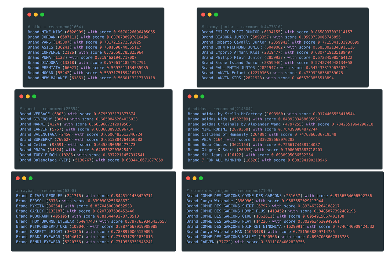
- Nike and Jordan is really interesting since they belong to the same parent company. Also, Nike recommendations seem to be decent, to say the least.
- Sister brands are recommended together, e.g. multiple Adidas collaborations and COMME DES GARÇONS labels.
- Great to see that every recommendation for Tommy Junior is indeed a Junior/Kids brand.
- Gucci and other related (I mean expensive) brands also together - Versace, Givenchy, Balenciaga, Prada and Burberry.
- I only own 2 sneaker brands: Adidas and Veja, so I’m quite happy with the Adidas recommendations even without Nike being there.
- Every recommendation for Rayban is also an eyewear brand.
Conclusion and next steps
I guess this was only the beginning of my Machine Learning journey. What I built here is really simple but, in a way, tackles an issue that I found that needed to be tackled. It had a real-world use-case, which was what I was looking for. On top of that, even though the model is simple, the results ended up being quite interesting.
The next step is setting up a pipeline that trains and deploys the model so that I can explore a little bit more the MLOps world. In fact, I have already this in place (it’s available in the same Github repository) and plan to write about the process soon.
My initial goal was to build a recommendations model based on collaborative filtering (it seems to be a lot more fun), so I might work on that in the future and combine both models into a Hybrid Recommendations System. Before doing so, I still have to figure out a way of evaluating the models to check whether the recommendations that it is making actually make any sense, other than my fashion judgement on which brands should be recommended together.
machine learning brand recommendations mle tfidf cosine similarity
2647 Words
2020-03-13 00:00 +0000