Probability Calibration
Please keep in mind that this will be a quite simple explanation of calibrated probabilities and how they are important. In order to learn more about how to use them for a specific type of model please refer to the References section below.
Let’s consider we are training a binary classification model that predicts whether a random photo has a dog or not, the predicted score will be a value from 0 to 1 (or 0 to 100%), ideally representing the probability of the image actually having a dog.
After training the model, regardless of its performance, we decide to test whether the value returned corresponds to the probability we are looking for. Our gut feeling certainly tells us that after having the model trained, if it returns a score of 0.5, it certainly means there’s a 50% chance of having a dog in the photo.
However, this is only true if, for a subset of photos with a predicted score of 0.5, 50% of them have dogs - when this happens we can say that the model returns calibrated probabilities, i.e. the predicted score represents the true likelihood of an event happening - in this case, the photo having a dog.
Probability calibration is the process of calibrating an ML model to return the true likelihood of an event. This is necessary when we need the probability of the event in question rather than its classification.
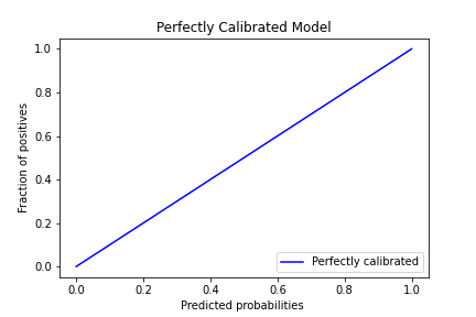
The plot above tries to represent this: on a calibrated model if there’s a predicted probability of 0.2, then the fraction of photos with dogs (positives) with this score will also be 0.2. The x-axis represents the average predicted probability, and the y-axis is the fraction of positives (photos with dogs).
Due to the nature of models, this is not what actually happens in practice most of the time. The next plot (from sklearn’s documentation), shows how the calibration of different model types (Logistic, Naive Bayes, SVC and Random Forest) would look in practice:
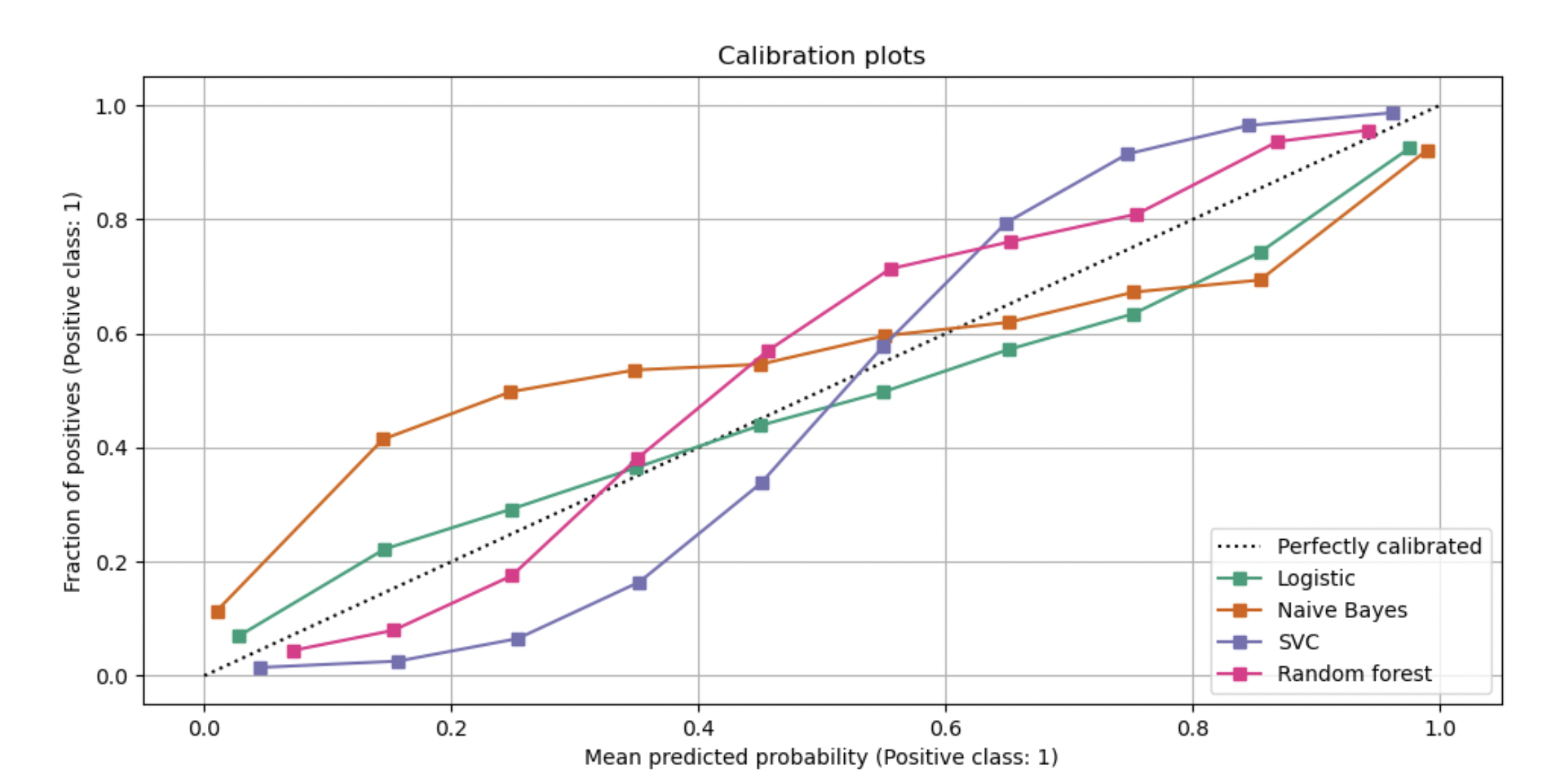
If we look closely at the calibration curve of the SVC and Naive Bayes models for a mean predicted probability of 0.2, we can easily see that the fraction of positives is actually quite far from 0.2 - it’s below 0.1 for SVC and above 0.4 for Naive Bayes. This means that when SVC returns a predicted probability of 0.2, less than 10% of photos would have dogs, and when Naive Bayes returns the same probability, more than 40% of photos would have dogs.
In order to have calibrated probabilities, our goal would be to have the calibration curve as close to the dashed line (Perfectly Calibrated) and only then we would be able to say that we are sure that a predicted probability of 0.2 means that there’s a 20% chance of a specific photo having a dog.